Drift diffusion models • tempodisco

library(tempodisco)

The drift diffusion model

Drift diffusion models (DDMs; Ratcliff, 1978) predict not only binary choices but also response times (RTs), and can be applied to intertemporal choice data (Peters & D’Esposito, 2020). DDMs model decision making as a process of noisy evidence accumulation in which the evidence $X$ begins at some value $\beta$ and evolves according to the stochastic differential equation

$\frac{d}{dt}X \sim \nu + \omega$

where $\delta$ is the drift rate, and $\omega$ is normally distributed noise with 0 mean and unit variance. Evidence begins accumulating after a non-decision period $\tau$ and is complete once $X$ reaches either 0 (meaning the delayed reward is chosen) or a threshold $\alpha$ (meaning the immediate reward is chosen). Thus, the model captures speed-accuracy tradeoffs: as $\alpha$ increases, decisions will be slower but more “accurate” (i.e., reflective of the decision maker’s relative preferences). This package relies on Wabersich and Vandekerckhove’s (2014) RWiener to compute first passage times for the diffusion process.

Following Peters & D’Esposito (2020), the drift rate is computed by multiplying the difference in subjective values by a scale factor $v$ :

$\delta = v\big( V_\text{imm} - V_\text{del}f(t;\mathbf{p})\big)$

where $V_\text{imm}$ is the value of the immediate reward, $V_\text{del}$ is the value of the delayed reward, and $f(t;\mathbf{p})$ is a discount function parameterized by $\mathbf{p}$ and evaluated at the delay of the delayed reward $t$ (i.e., $t$ in this equation does not refer to time within a single decision trial as in the previous equation).

Fitting drift diffusion models

Often, extreme RTs are first excluded, using either absolute or relative cutoffs. Here, we will exclude the fastest 2.5% and slowest 2.5% of responses.

data("td_bc_single_ptpt")
rt_cutoffs <- quantile(td_bc_single_ptpt$rt, c(0.025, 0.975))
td_bc_single_ptpt <- subset(td_bc_single_ptpt, rt > rt_cutoffs[1] & rt < rt_cutoffs[2])

Next, we can fit a drift diffusion model. Here, for the sake of speed, we are providing starting values for the parameters that are close to optimal and are only testing the exponential discount function.

ddm <- td_ddm(td_bc_single_ptpt, discount_function = 'exponential',
              v_par_starts = 0.01,
              beta_par_starts = 0.5,
              alpha_par_starts = 3.5,
              tau_par_starts = 0.9)
print(ddm)
#> 
#> Temporal discounting drift diffusion model
#> 
#> Discount function: exponential
#> Coefficients:
#> 
#>           k           v        beta       alpha         tau 
#> 0.009518797 0.008810812 0.574805668 3.462444316 0.946851140 
#> 
#> "none" transform applied to drift rates.
#> 
#> ED50: 72.8187765186714
#> AUC: integrate() failed to compute AUC with error: "unused argument (verbose = FALSE)"
#> BIC: 236.382759846412

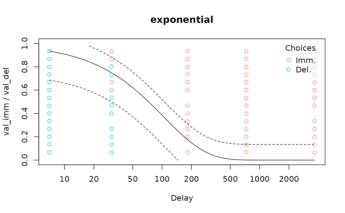
As we can see, parameters are estimated not only for the discount function ( $k$ ), but also for the DDM ( $v$ , $\beta$ , $\alpha$ and $\tau$ ). These can be extracted using coef() to collect for group-level analysis (see the vignette “Analyzing data from multiple participants”). As with other model classes (td_bcnm, td_bclm), we can plot the resulting discount function:

plot(ddm, log = 'x', verbose = F, p_lines = c(0.25, 0.75))

Here the gaps correspond to very fast or slow decisions that we excluded.

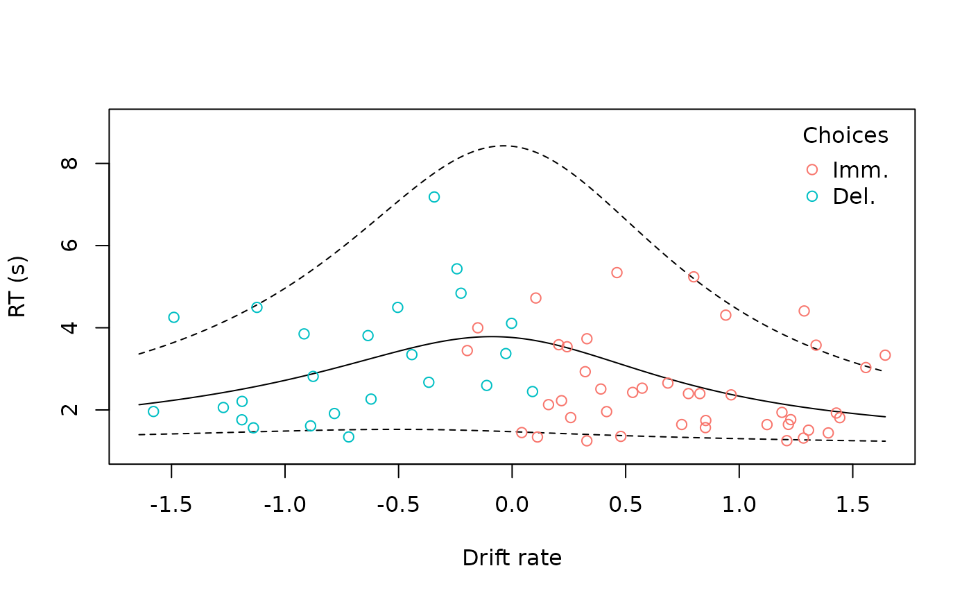
Moreover, because DDMs model RTs, we can compare predicted RTs to the actual data:

predicted_rts <- predict(ddm, type = 'rt')
cor.test(predicted_rts, ddm$data$rt)
#> 
#>  Pearson's product-moment correlation
#> 
#> data:  predicted_rts and ddm$data$rt
#> t = 2.6422, df = 64, p-value = 0.01034
#> alternative hypothesis: true correlation is not equal to 0
#> 95 percent confidence interval:
#>  0.07746325 0.51644776
#> sample estimates:
#>       cor 
#> 0.3136161

As expected, they are correlated. To compare these visually, we can plot() the DDM with the argument type = "rt":

plot(ddm, type = 'rt', q_lines = c(0.05, 0.95), ylim = c(1, 9))

This displays both the predicted RTs from the model and a 90% quantile-based confidence interval

Fontanesi et al. (2019) suggest applying a sigmoid transform to drift rates according the the following equation, which is reported by Peters & D’Esposito (2020) to improve model fit for intertemporal choice data:

$\delta' = v_\text{max} \left(\frac{2}{1 + \exp\{-\delta\}} - 1\right)$

We can incorporate this into the model using the argument drift_transform = "sigmoid":

ddm_sig <- td_ddm(td_bc_single_ptpt, discount_function = 'exponential', drift_transform = 'sigmoid',
              v_par_starts = 0.01,
              beta_par_starts = 0.5,
              alpha_par_starts = 3.5,
              tau_par_starts = 0.9)
print(BIC(ddm))
#> [1] 236.3828
print(BIC(ddm_sig))
#> [1] 230.1002

Sure enough, the model with the sigmoid transform performs better per the Bayesian information criterion. Plotting the probability of choosing the immediate reward against the drift rate, we can see that many datapoints are pushed to either extreme, creating good separation between cases where the immediate versus delayed rewards were chosen.

plot(ddm_sig, type = 'link')