Getting started

library(tempodisco)

This vignette briefly goes over the main steps involved in analyzing delay discounting data. These topics are covered in greater depth in other vignettes and in the documentation of the relevant functions.

Loading data

tempodisco includes several example datasets. We will load one example from a simulated “adjusting amounts” procedure (Frye et al., 2016), and one from a procedure in which choices were not structured according to such a procedure.

data("adj_amt_sim") # Load simulated choice data from an adjusting amounts procedure
head(adj_amt_sim)
#>   del val_del val_imm imm_chosen trial_idx
#> 1   7     800     400      FALSE         1
#> 2   7     800     600      FALSE         2
#> 3   7     800     700      FALSE         3
#> 4   7     800     750      FALSE         4
#> 5   7     800     775      FALSE         5
#> 6  30     800     400      FALSE         6
data("td_bc_single_ptpt") # Load choice data from a non-adjusting-amounts experiment
head(td_bc_single_ptpt)
#>                                   id val_imm val_del       del imm_chosen    rt
#> 1 61dcacaa5ed72-dd-61dcb234e8a1c.txt     112     187   30.4167      FALSE 5.435
#> 2 61dcacaa5ed72-dd-61dcb234e8a1c.txt      50     187   30.4167      FALSE 1.913
#> 3 61dcacaa5ed72-dd-61dcb234e8a1c.txt      37     186 3652.5000       TRUE 2.931
#> 4 61dcacaa5ed72-dd-61dcb234e8a1c.txt      28     211  182.5000      FALSE 7.639
#> 5 61dcacaa5ed72-dd-61dcb234e8a1c.txt      53     197  182.5000       TRUE 2.129
#> 6 61dcacaa5ed72-dd-61dcb234e8a1c.txt      98     184  730.5000       TRUE 1.569

For each dataset, there are rows containing the values of the immediate and delayed rewards, the delay of the delayed reward, and whether the immediate reward was chosen. To use the functions in tempodisco, your own data will need these same columns named in the same way.

Computing indifference points

For the adjusting amounts data, we can use the adj_amt_indiffs function to compute indifference points at each delay:

indiff_data <- adj_amt_indiffs(adj_amt_sim)
head(indiff_data)
#>   del   indiff
#> 1   7 0.984375
#> 2  30 0.859375
#> 3  90 0.046875
#> 4 180 0.453125
#> 5 360 0.015625

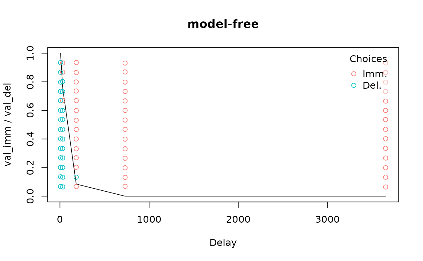
For non-adjusting-amounts data, we can use a form of logistic regression that models each indifference point as the point at which a participant has a 50% estimated probability of selecting the immediate or delayed reward:

indiff_mod <- td_bcnm(td_bc_single_ptpt, discount_function = 'model-free')
plot(indiff_mod, verbose = F)

Data quality checks

We can test for non-systematic discounting per the criteria of Johnson & Bickel (2008) using the nonsys function:

print(nonsys(indiff_data)) # Fails criterion 1 (monotonicity)
#>    C1    C2 
#>  TRUE FALSE
print(nonsys(indiff_mod))
#>    C1    C2 
#> FALSE FALSE

Measuring discounting

To quantify discounting given a set of indifference points, we can use the “area under the curve” measure (Myerson et al., 2001). The lower this measure is, the steeper an individual’s delay discounting.

AUC(indiff_data)
#> [1] 0.3333984
AUC(indiff_mod)
#> [1] 0.03146756

Fitting discount functions

Fitting a discount function to a set of indifference points can be done using the td_ipm function:

hyperbolic_mod <- td_ipm(indiff_data, discount_function = 'hyperbolic')
plot(hyperbolic_mod)

coef(hyperbolic_mod)
#>          k 
#> 0.01767284

In contrast, fitting a discount function to choice-level data involves a form of logistic regression where, as before, the indifference points (determined by a discount function) are the points where the individual has a 50% estimated probability of selecting the immediate vs delayed reward.

hyperbolic_mod <- td_bcnm(td_bc_single_ptpt, discount_function = 'hyperbolic')
plot(hyperbolic_mod, verbose = F)

coef(hyperbolic_mod)
#>          k      gamma 
#> 0.01728415 0.06743971

From here, we can extract the $k$ values from the best-fitting hyperbolic discount curves for each participant and use these as a measure of discounting (higher $k$ means steeper discounting).